Machine Learning 실습예제 - linear regression
Modeling 구성
Linear regression modeling
import pandas as pd
import matplotlib.pyplot as plt
import statsmodels
# load data from the Univ. of East Anglia Climate Research Unit (CRU)
# (https://crudata.uea.ac.uk/cru/data/hrg/cru_ts_4.03/).

# The following variables are available
# tmp - Temperature
# cld - Cloud cover
# dtr - Diurnal temperature range
# frs - Ground frost frequency
# pet - potential evapotranspiration
# pre - precipitation
# vap - vapor pressure
# wet - Wet day frequency
# This is the base URL where the data are stored:
base_url = 'https://crudata.uea.ac.uk/cru/data/hrg/cru_ts_4.05/crucy.2103081329.v4.05/countries/VAR/crucy.v4.05.1901.2020.all.VAR.per'

# Load the temperature data. The field "ANN" contains the annual average.
url = base_url.replace('VAR','tmp')
data_tmp = pd.read_fwf(url, skiprows=3) # Read "fixed-width format"
data_tmp = data_tmp[['YEAR','ANN']]
data_tmp.head()

# 어떤식으로 작동하는지는 모름
| YEAR | ANN | |
|---|---|---|
| 0 | 1901 | 13.0 |
| 1 | 1902 | 12.8 |
| 2 | 1903 | 12.8 |
| 3 | 1904 | 12.8 |
| 4 | 1905 | 12.9 |
# Now loop through each of the variables and load each one.
# Append them to each other to create a joint dataframe containing
# all of the desired variables.

# Make a list of the variables we want to examine:
variables = ['tmp','wet','frs','cld']

data_list = []
for var in variables:
    url = base_url.replace('VAR',var)
    data_var = pd.read_fwf(url, skiprows=3) # Read "fixed-width format"
    data_var = data_var[['YEAR','ANN']]

    # Rename the "ANN" column (annual)
    data_var = data_var.rename(columns={'ANN':var})

    # Set "YEAR" to be the index
    data_var = data_var.set_index('YEAR')
    data_list.append(data_var)

data = data_list[0].join(data_list[1:]).reset_index()
data.head()

# 어떤식으로 작동하는지는 모름
| YEAR | tmp | wet | frs | cld | |
|---|---|---|---|---|---|
| 0 | 1901 | 13.0 | 110.5 | 99.4 | 54.7 |
| 1 | 1902 | 12.8 | 110.1 | 101.6 | 54.6 |
| 2 | 1903 | 12.8 | 111.0 | 101.2 | 54.9 |
| 3 | 1904 | 12.8 | 110.7 | 100.9 | 54.7 |
| 4 | 1905 | 12.9 | 111.1 | 101.3 | 55.0 |
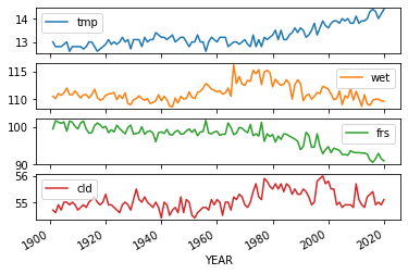
# 각각의 column들을 x값에 year를 넣고 plot
data.plot(x='YEAR',subplots=True)
array([<AxesSubplot:xlabel='YEAR'>, <AxesSubplot:xlabel='YEAR'>,
       <AxesSubplot:xlabel='YEAR'>, <AxesSubplot:xlabel='YEAR'>],
      dtype=object)
# ols (lilnear regression) import
from statsmodels.formula.api import ols
# 매해 온도 변화 plot으로 나타냄
plt.plot(data["YEAR"],data["tmp"], '.')
plt.xlabel("Time in Year")
plt.ylabel("Celcius")
Text(0, 0.5, 'Celcius')
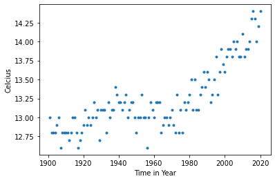
They appear correlated posivitly which means temperature increases as time goes.Their relationship is linear.
매년 온도가 증가하는 것으로 보이므로 x 변수 year와 y 변수 temperature의 관계가 linear regression (선형 회귀)로 보임
# ols function을 사용해서 model을 만듬
model = ols(formula='tmp ~ 1+ YEAR',data = data)

# Fit the model
model = model.fit()

print(model.summary())
                            OLS Regression Results
==============================================================================
Dep. Variable:                    tmp   R-squared:                       0.665
Model:                            OLS   Adj. R-squared:                  0.662
Method:                 Least Squares   F-statistic:                     234.1
Date:                Thu, 13 May 2021   Prob (F-statistic):           8.65e-30
Time:                        09:27:23   Log-Likelihood:                -2.7541
No. Observations:                 120   AIC:                             9.508
Df Residuals:                     118   BIC:                             15.08
Df Model:                           1
Covariance Type:            nonrobust
==============================================================================
                 coef    std err          t      P>|t|      [0.025      0.975]
------------------------------------------------------------------------------
Intercept     -6.4968      1.290     -5.036      0.000      -9.052      -3.942
YEAR           0.0101      0.001     15.301      0.000       0.009       0.011
==============================================================================
Omnibus:                        1.569   Durbin-Watson:                   0.732
Prob(Omnibus):                  0.456   Jarque-Bera (JB):                1.551
Skew:                          -0.269   Prob(JB):                        0.460
Kurtosis:                       2.856   Cond. No.                     1.11e+05
==============================================================================

Notes:
[1] Standard Errors assume that the covariance matrix of the errors is correctly specified.
[2] The condition number is large, 1.11e+05. This might indicate that there are
strong multicollinearity or other numerical problems.
point estimate of intercept: -6.4968
point estimate of ‘year’: 0.0101
# 모델링의 lilne을 기존 scatter plot에 표시

data["predict"] = model.predict()
plt.plot(data["YEAR"],data["tmp"], '.')
plt.plot(data["YEAR"], data["predict"])
plt.xlabel("YEAR")
plt.ylabel("tmp")
Text(0, 0.5, 'tmp')
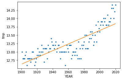
모델의 라인을 보면 x value인 year가 증가할수록 y value인 온도도 증가하는 것으로 보임. 기울기가 positive인것으로 보아 매년 지구의 온도가 올라감.
model.pvalues
Intercept    1.730160e-06
YEAR         8.653127e-30
dtype: float64
p value가 0에 가깝기 때문에 year는 statistically significant한 변수임
# 지구 온도와 구름의 상관관계를 나타내는 모델
model_cld = ols(formula='tmp ~ 1 + cld',data = data)

# Fit the model:
model_cld = model_cld.fit()

print(model_cld.summary())
                            OLS Regression Results
==============================================================================
Dep. Variable:                    tmp   R-squared:                       0.076
Model:                            OLS   Adj. R-squared:                  0.068
Method:                 Least Squares   F-statistic:                     9.731
Date:                Thu, 13 May 2021   Prob (F-statistic):            0.00228
Time:                        09:35:30   Log-Likelihood:                -63.599
No. Observations:                 120   AIC:                             131.2
Df Residuals:                     118   BIC:                             136.8
Df Model:                           1
Covariance Type:            nonrobust
==============================================================================
                 coef    std err          t      P>|t|      [0.025      0.975]
------------------------------------------------------------------------------
Intercept     -5.2952      5.942     -0.891      0.375     -17.063       6.472
cld            0.3366      0.108      3.120      0.002       0.123       0.550
==============================================================================
Omnibus:                       17.828   Durbin-Watson:                   0.284
Prob(Omnibus):                  0.000   Jarque-Bera (JB):               21.160
Skew:                           1.016   Prob(JB):                     2.54e-05
Kurtosis:                       3.320   Cond. No.                     8.65e+03
==============================================================================

Notes:
[1] Standard Errors assume that the covariance matrix of the errors is correctly specified.
[2] The condition number is large, 8.65e+03. This might indicate that there are
strong multicollinearity or other numerical problems.
point estimate of intercept: -5.2952
point estimate of ‘cld’: 0.3366
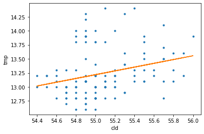
#  모델링의 lilne을 기존 scatter plot에 표시
data["predict_cld"] = model_cld.predict()
plt.plot(data["cld"],data["tmp"], '.')
plt.plot(data["cld"], data["predict_cld"])
plt.xlabel("cld")
plt.ylabel("tmp")
Text(0, 0.5, 'tmp')
model_cld.pvalues
Intercept    0.374691
cld          0.002277
dtype: float64
cld 변수의 p value가 0.5보다 크지 않으므로 statistically significant한 변수라고 할 수 있음.
식으로 나타내면 formula: y = 0.3366x1 - 5.2952 표현할수 있음
# 지구 온도와 여러가지 parameters과의 상관관계를 나타내는 모델
model_multiple = ols(formula='tmp ~ 1 + wet + frs + cld',data = data)

# Fit the model:
model_multiple = model_multiple.fit()

print(model_multiple.summary())
                            OLS Regression Results
==============================================================================
Dep. Variable:                    tmp   R-squared:                       0.943
Model:                            OLS   Adj. R-squared:                  0.941
Method:                 Least Squares   F-statistic:                     637.5
Date:                Thu, 13 May 2021   Prob (F-statistic):           7.04e-72
Time:                        09:38:08   Log-Likelihood:                 103.33
No. Observations:                 120   AIC:                            -198.7
Df Residuals:                     116   BIC:                            -187.5
Df Model:                           3
Covariance Type:            nonrobust
==============================================================================
                 coef    std err          t      P>|t|      [0.025      0.975]
------------------------------------------------------------------------------
Intercept     28.5361      1.753     16.277      0.000      25.064      32.008
wet           -0.0267      0.007     -3.573      0.001      -0.042      -0.012
frs           -0.1464      0.004    -37.902      0.000      -0.154      -0.139
cld            0.0355      0.035      1.026      0.307      -0.033       0.104
==============================================================================
Omnibus:                        0.615   Durbin-Watson:                   1.917
Prob(Omnibus):                  0.735   Jarque-Bera (JB):                0.727
Skew:                          -0.057   Prob(JB):                        0.695
Kurtosis:                       2.636   Cond. No.                     2.91e+04
==============================================================================

Notes:
[1] Standard Errors assume that the covariance matrix of the errors is correctly specified.
[2] The condition number is large, 2.91e+04. This might indicate that there are
strong multicollinearity or other numerical problems.
model_multiple.pvalues
Intercept    9.866650e-32
wet          5.159167e-04
frs          3.491024e-67
cld          3.068349e-01
dtype: float64
모든 parameters의 p-value가 0에 가까우므로 reject null hypothesis와 모든 parameters는 statistically significant한 변수들이다.
multiple linear regression으로 모델링 한것과 sigle linear regression으로 모델링한것의 point estimate가 다른 것으로 보아 각각의 parameters들은 서로 영향을 끼치는 것을 알 수 있다.
# 모델의 prediction
data["predict_multiple"] = model_multiple.predict()
plt.plot(data["tmp"],data["predict_multiple"], '.')
[<matplotlib.lines.Line2D at 0x195cf567190>]
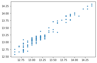
from scipy.stats import pearsonr

corr = pearsonr(data['tmp'], data['predict_multiple'])
corr
(0.9709853571622034, 3.6172955865432555e-75)
# 상관 계수 pearson r (correlation coefficient)
corr[0]
0.9709853571622034
correlation coefficient가 양수 인것으로 보아 각각의 parameter들은 서로 linear한 관계를 가지고 있다 (ex. x1이 증가하면 x2도 증가함)
- fraction of variance of y : R^2
- R^2가 0.943 (in the summary of model)이므로 변수들의 설명력이 94.3% 이고 y에 대해well-described된 parameters를 가진 모델로 설명할 수 있다